Wednesday, November 30, 2011

A Python Metaclass for "extra bad" errors in Google App Engine

So now here we are, having tried to handle errors in Google App Engine...and failed all because silly DeadlineExceededError jumps over Exception in the inheritance chain and goes right for BaseException. How can we catch these in our handlers while staying Pythonic*?

First and foremost, in the case of a timeout, we need to explicitly catch a DeadlineExceededError. To do so, we can use a decorator (hey, that's Pythonic) in each and every handler for each and every HTTP verb. (Again, prepare yourselves, a bunch of code is about to happen. See the necessary imports at the bottom of the post.)
def deadline_decorator(method):

    def wrapped_method(self, *args, **kwargs):
        try:
            method(self, *args, **kwargs)
        except DeadlineExceededError:
            traceback_info = ''.join(format_exception(*sys.exc_info()))
            email_admins(traceback_info, defer_now=True)

            serve_500(self)

    return wrapped_method
Unfortunately, having to manually
is not so Pythonic. At this point I was stuck and wanted to give up, but asked for some advice on G+ and actually got what I needed from the all knowing Ali Afshar. What did I need? Metaclasses.

Before showing the super simple metaclass I wrote, you need to know one thing from StackOverflow user Kevin Samuel:
The main purpose of a metaclass is to change the class automatically, when it's created.
With the __new__ method, the type object in Python actually constructs a class (which is also an object) by taking into account the name of the class, the parents (or bases) and the class attritubutes. So, we can make a metaclass by subclassing type and overriding __new__:
class DecorateHttpVerbsMetaclass(type):

    def __new__(cls, name, bases, cls_attr):
        verbs = ['get', 'post', 'put', 'delete']
        for verb in verbs:
            if verb in cls_attr and isinstance(cls_attr[verb], function):
                cls_attr[verb] = deadline_decorator(cls_attr[verb])

        return super(DecorateHttpVerbsMetaclass, cls).__new__(cls, name,
                                                              bases, cls_attr)
In DecorateHttpVerbsMetaclass, we look for four (of the nine) HTTP verbs, because heck, only seven are supported in RequestHandler, and we're not that crazy. If the class has one of the verbs as an attribute and if the attribute is a function, we decorate it with deadline_decorator.

Now, we can rewrite our subclass of RequestHandler with one extra line:
class ExtendedHandler(RequestHandler):
    __metaclass__ = DecorateHttpVerbsMetaclass

    def handle_exception(self, exception, debug_mode):
        traceback_info = ''.join(format_exception(*sys.exc_info()))
        email_admins(traceback_info, defer_now=True)

        serve_500(self)
By doing this, when the class ExtendedHandler is built (as an object), all of its attributes and all of its parent classes (or bases) attributes are checked and possibly updated by our metaclass.

And now you and James Nekbehrd can feel like a boss when your app handles errors.

Imports:
from google.appengine.api import mail
from google.appengine.ext.deferred import defer
from google.appengine.ext.webapp import RequestHandler
from google.appengine.runtime import DeadlineExceededError
import sys
from traceback import format_exception
from SOME_APP_SPECIFIC_LIBRARY import serve_500
from LAST_POST import email_admins
*Pythonic:
An idea or piece of code which closely follows the most common idioms of the Python language, rather than implementing code using concepts common to other languages.
Notes:
  • Using grep -r "Exception)" . | grep "class " I have convinced myself (for now) that the only errors AppEngine will throw that do not inherit from Exception are DeadlineExceededError, SystemExit, and KeyboardInterrupt so that is why I only catch the timeout.
  • You can also use webapp2 to catch 500 errors, even when handle_exception fails to catch them.

Disclaimer: Just because you know what a metaclass is doesn't mean you should use one:
  • "Don't do stuff like this though, what is your use case?" -Ali Afshar
  • "Metaclasses are deeper magic than 99% of users should ever worry about. If you wonder whether you need them, you don't (the people who actually need them know with certainty that they need them, and don't need an explanation about why)." -Python Guru Tim Peters
  • "The main use case for a metaclass is creating an API." -Kevin Samuel

Sunday, November 27, 2011

Handling errors in Google App Engine...and failing

After spending a nontrivial amount of my nights and weekends working on an AppEngine app, I wanted a good way to monitor the logs without checking in on them every day. After a particularly frustrating weekend of updates that exposed unnoticed bugs that had yet to be triggered by the app, I set out to find such a way. I set out to find a Pythonic* way.

Since I knew the App Engine Mail API was super easy to configure,  I figured I would just email myself every time there was an exception, before serving my default 500 error page. To do so, I just needed to subclass the default RequestHandler with my own handle_exception method. (OK, prepare yourselves, a bunch of code is about to happen. See the necessary imports at the bottom of the post.)
class ExtendedHandler(RequestHandler):

    def handle_exception(self, exception, debug_mode):
        traceback_info = ''.join(format_exception(*sys.exc_info()))
        email_admins(traceback_info, defer_now=True)

        serve_500(self)
Awesome! By making all my handlers inherit from ExtendedHandler, I can use the native Python modules traceback and sys to get the traceback and my handy dandy
def email_admins(error_msg, defer_now=False):
    if defer_now:
        defer(email_admins, error_msg, defer_now=False)
        return

    sender = 'YOUR APP Errors <errors@your_app_id_here.appspotmail.com>'
    to = 'Robert Admin <bob@example.com>, James Nekbehrd <jim@example.com>'
    subject = 'YOUR APP Error: Admin Notify'
    body = '\n'.join(['Dearest Admin,',
                      '',
                      'An error has occurred in YOUR APP:',
                      error_msg,
                      ''])

    mail.send_mail(sender=sender, to=to,
                   subject=subject, body=body)
to send out the email in the deferred queue** so as not to hold up the handler serving the page. Mission accomplished, right? WRONG!

Unfortunately, handle_exception only handles the "right" kind of exceptions. That is, exceptions which inherit directly from Python's Exception. From the horse's mouth:
Exceptions should typically be derived from the Exception class, either directly or indirectly.
But. But! If the app fails because a request times out, a DeadlineExceededError is thrown and handle_exception falls on its face. Why? Because DeadlineExceededError inherits directly from Exception's parent class: BaseException.  (Gasp)

It's OK little ones, in my next post I explain how I did it while keeping my code Pythonic by using metaclasses.

Imports:
from google.appengine.api import mail
from google.appengine.ext.deferred import defer
from google.appengine.ext.webapp import RequestHandler
import sys
from traceback import format_exception
from SOME_APP_SPECIFIC_LIBRARY import serve_500
*Pythonic:
An idea or piece of code which closely follows the most common idioms of the Python language, rather than implementing code using concepts common to other languages.
**Deferred Queue: Make sure to enable the deferred library in your app.yaml by using deferred: on in your builtins.

Thursday, November 17, 2011

Quick and Dirty: Santa's Coming

I have been wanting to write a post for awhile, but was travelling for a work event and while on the road I decided to be lazy.

Since I just so happen to use a few GData APIs occasionally in my day to day work, most of the post ideas revolve around quirky things I have done or want to do with the APIs. Also, due to my obscene love for Python, all my mashups seem to end up using the Python Client for GData.

Back-story: As I was finalizing travel and gifts for my winter holiday back home, I called an old friend to let him know I'd be home in 40 days. After relaying this information to a few other people, I noted to my girlfriend that it would be nice if a computer would remind me of the count every day. This is where this quick and dirty pair of scripts come in to remind me when Santa is coming.

Pre-work — Account Settings: To allow an app to make requests on my behalf, I signed up to Manage my Domain for use with Google Apps, etc. For illustration purposes, let's say I used http://example.com (in reality, I used a pre-existing App of mine, I really just needed an OAuth token for one time use, no real safety concerns there). After adding this domain in the management page, I am able to get my "OAuth Consumer Key" and "OAuth Consumer Secret" which we'll say are EXAMPLE_KEY and EXAMPLE_SECRET in this example. Also in the management page, I set my "OAuth 2.0 Redirect URIs" and made sure my app can serve that page (even if it is a 404). Again for illustration, let's pretend I used http://example.com/verify.

After doing this settings pre-work, I have two scripts to do the work for me.

First script — get the OAuth Token:
import gdata.calendar.client
import gdata.gauth

gcal = gdata.calendar.client.CalendarClient()
oauth_callback = 'http://example.com/verify'
scopes = ['https://www.google.com/calendar/feeds/']
consumer_key = 'EXAMPLE_KEY'
consumer_secret = 'EXAMPLE_SECRET'
request_token = gcal.get_oauth_token(scopes, oauth_callback,
                                     consumer_key, consumer_secret)
out_str = ('Please visit https://www.google.com/accounts/OAuthAuthorize'
           'Token?hd=default&oauth_token=%s' % request_token.token)
print out_str
follow = raw_input('Please entry the follow link after authorizing:\n')
gdata.gauth.authorize_request_token(request_token, follow)
gcal.auth_token = gcal.get_access_token(request_token)
print 'TOKEN:', gcal.auth_token.token
print 'TOKEN_SECRET:', gcal.auth_token.token_secret
This script "spoofs" the OAuth handshake by asking the user (me) to go directly to the OAuth Authorize page. After doing so and authorizing the App, I am redirected to http://example.com/verify with query parameters for oauth_verifier and oauth_token. These are then used by the gauth section of the GData library to finish the OAuth handshake. Once the handshake is complete, the script prints out a necessary token and token secret to be used by the second script. I would advise piping the output to a file, augmenting the script to write them to a file, or writing these down (this is a joke, please don't write down 40 plus character goop that was produced by your computer). For the next script, let's pretend our token is FAKE_TOKEN and our token secret is FAKE_TOKEN_SECRET.

Second script — insert the events:
# General libraries
from datetime import date
from datetime import timedelta

# Third-party libraries
import atom
import gdata.gauth
import gdata.calendar.client
import gdata.calendar.data

gcal = gdata.calendar.client.CalendarClient()
auth_token = gdata.gauth.OAuthHmacToken(consumer_key='EXAMPLE_KEY',
                                        consumer_secret='EXAMPLE_SECRET',
                                        token='FAKE_TOKEN',
                                        token_secret='FAKE_TOKEN_SECRET',
                                        auth_state=3)
gcal.auth_token = auth_token

today = date.today()
days_left = (date(year=2011, month=12, day=23) - today).days

while days_left >= 0:
    event = gdata.calendar.data.CalendarEventEntry()
    if days_left > 1:
        msg = '%s Days Until Home for Christmas' % days_left
    elif days_left == 1:
        msg = '1 Day Until Home for Christmas'
    elif days_left == 0:
        msg = 'Going Home for Christmas'
    event.title = atom.data.Title(msg)

    # When
    start_time = '2011-%02d-%02dT08:00:00.000-08:00' % (today.month, today.day)
    end_time = '2011-%02d-%02dT09:00:00.000-08:00' % (today.month, today.day)
    event.when.append(gdata.calendar.data.When(
        start=start_time,
        end=end_time,
        reminder=[gdata.data.Reminder(hours='1')]))

    gcal.InsertEvent(event)

    today += timedelta(days=1)
    days_left -= 1
This script first authenticates by using the key/secret pair for the application (retrieved from the settings page) and the key/secret pair for the user token (that we obtained from the first script). To authenticate, we explicitly construct an HMAC-SHA1 signed token in the final auth state (3) of two-legged OAuth and then set the token on our calendar client (gcal).

After authenticating, we start with today and figure out the number of days in the countdown given my return date of December 23, 2011. With these in hand, we can loop through until there are no days left, creating a CalendarEventEntry with title as the number of days left in the countdown and occurring from 8am to 9am PST (UTC -8). Notice also I include a gdata.data.Reminder so I get an email at 7am every morning (60 minutes before the event) updating my brain on the length of the countdown!

Cleanup: Be sure to go to your issued tokens page and revoke access to the App (e.g. http://example.com) after doing this to avoid any unwanted security issues.

References: I have never read this, but I'm sure the documentation on Registration for Web-Based Applications is very helpful.

Notes:
  • You can annoy other people by inviting them to these events for them as well. To do so, simply add the following two lines before inserting the event
    who_add = gdata.calendar.data.EventWho(email='name@mail.com')
    event.who.append(who_add)
  • Sometimes inserting an item results in a RedirectError, so it may be safer to try the insert multiple times with a helper function such as the following:
    def try_insert(attempts, gcal, event):
        from time import sleep
        from gdata.client import RedirectError
    
        while attempts > 0:
          try:
              gcal.InsertEvent(event)
              break
          except RedirectError:
              attempts -= 1
              sleep(3)
              pass
    
        if attempts == 0:
            print 'Insert "%s" failed' % event.title.text
  • In what I swear was a complete coincidence, v3 of the Calendar API was announced today. I will try to use the new documentation to redo this quick and dirty example with v3.

Wednesday, October 5, 2011

Protecting Sensitive Information in Public Git Repositories

On the (much too early) bus to work this morning, I was reading my Twitter feed and saw an interesting question from Rob Hawkes:
Rob Hawkes @robhawkes
Rob Hawkes

How do you handle config files in your apps when you use Git? I keep accidentally adding config files with sensitive data to Git. :(
Rob's Twitter followers made all kinds of recommendations and Rob eventually decided it was a solved problem, declaring "Best method I've found so far is creating a temporary config file and keeping that in git, then .gitignoring the real one." and then "Thanks for the config file tips! In the end I went with a "config.example.js" file stored in Git and a "config.js" file that is ignored." For those following along at home, they mean the same thing.

As Rob was probably intending, this can be used for deploying an app on your personal server, or for a sample App on a PaaS like Google App Engine or Heroku. When testing such an app, the ability to have a native environment locally is a huge convenience, but the overhead of remembering which private keys need to be hidden is a headache and sometimes completely neglected. But it shouldn't be, because git never forgets!

Anyone who has used git for any substantial amount of time probably initially conceived of this hack when on first thought. (This is no insult to Rob, just the inevitability of the pattern.) But, by the time Rob posted his solution, I had moved on from this and came up a solution that I think does the trick a bit more thoroughly. I envisioned a solution which assumes people who checkout my code will want to keep their config in a specified path that is already in the repo; of course, I also wanted to share this with the interwebs.

Anyhow, this is quick and dirty. First, create config.js and _config.js in the root directory of your git repository (the same directory that .git lives in). I intend config.js to be the local copy with my actual passwords and keys and _config.js to hold the master contents that actually show up in the public repo. For example, the contents of config.js are:
var SECRET = 'Nnkrndkmn978489MDkjw';
and the contents of _config.js are:
var SECRET = 'SECRET';
Since I don't want a duplicate in my repo, I put a rule in my .gitignore file to ignore _config.js. (For those unfamiliar, this can be done just by including _config.js on its own line in the .gitignore file.) After doing so, I set up two git hooks, a pre-commit and post-commit hook.

To "install" the hooks, just add the files pre-commit and post-commit to the .git/hooks subdirectory in your repo. They are nearly identical files, with a one-line difference. Both files simply swap the contents of config.js and _config.js, while pre-commit also adds config.js to the changelist. First I'll give you the contents of pre-commit, and then explain why it's cool/safe:
#!/usr/bin/env python

import os

hooks_dir = os.path.dirname(os.path.abspath(__file__))
relative_dir = os.path.join(hooks_dir, '../..')
project_root = os.path.abspath(relative_dir)

git_included_config = os.path.join(project_root, 'config.js')
confidential_config = os.path.join(project_root, '_config.js')

with open(git_included_config, 'rU') as fh:
  git_included_contents = fh.read()

with open(confidential_config, 'rU') as fh:
  confidential_contents = fh.read()

with open(git_included_config, 'w') as fh:
  fh.write(confidential_contents)

with open(confidential_config, 'w') as fh:
  fh.write(git_included_contents)

os.system('git add %s' % git_included_config)
(Also note the contents of post-commit are exactly the same, except without the final statement: os.system('git add %s' % git_included_config).)

So what is happening in this file:
  1. Uses the Python os module to determine the absolute path to the root directory in your project by using the absolute path of the hook file, backing up two directories and again find that absolute path.
  2. Determines the two files which need to swap contents
  3. Loads the contents into string variables and then writes them to the opposite files
  4. (only in pre-commit) Adds the included file to the changelist before the commit occurs.
Step 4 is actually the secret sauce. It puts cleaned, non-sensitive data into the checked in config.js file and then updates the changelist before making a commit, to ensure only the non-sensitive data goes in. Though you could do this yourself by making an initial commit with clean data and then never git adding the file with your actual data, these hooks prevent an accident and allow you to update your local _config.js file with more fields as your config spec changes.

But wait bossylobster, you say, what if one of the hooks doesn't occur? You are right! As  pre-commit stands above, if the changelist is empty we have problems. Since the pre-commit hook changes  config.js to the same value in HEAD, git will tell us either "nothing to commit" or "no changes added to commit". In this case, the commit will exit and the post-commit hook will never occur. This is very bad, since the contents of config.js and _config.js will be switched but not switched back. So, to account for this, we need to append the following code to the end of pre-commit:
with os.popen('git st') as fh:
  git_status = fh.read()

if ('nothing to commit' in git_status or
    'no changes added to commit' in git_status or
    'nothing added to commit' in git_status):
  import sys

  msg = '# From pre-commit hook: No commit necessary, ' \
        'sensitive config unchanged. #'
  hash_head = '#' * len(msg)
  print ('%s\n%s\n%s\n\n' % (hash_head, msg, hash_head)),

  with open(git_included_config, 'w') as fh:
    fh.write(git_included_contents)

  with open(confidential_config, 'w') as fh:
    fh.write(confidential_contents)

  sys.exit(1)
For final versions see the pre-commit and post-commit files. Thanks again to Rob Hawkes for the idea/work break over lunch!

Update: One of Rob's followers, Paul King, found and tweeted a very different alternative that is also pretty cool. Check out the post he found by Rob Wilkerson.

UpdateI swapped out a screen shot of the tweet for a CSS-ified version, inspired by and based on a design used on Mashable.

Update: Some change in git causes empty commits to be allowed. I either didn't notice this before or it just showed up in git. So I added sys.exit(1) to force the pre-commit script to fail when nothing is changed and added a check for the phrase nothing added to commit as well.

Monday, August 29, 2011

Finding (Fibonacci) Golden Nuggets Part 2

This is the mostly code second half of a two part post that delivers on a promise of meaningful uses of some theory I overviewed in my last set of posts. If you see words like topograph, river, and base and you aren't sure what I mean, you may want to read that last set of posts.

In the first half of this post, I outlined a solution to Project Euler problem 137 and will continue with the solution here. Stop reading now if you don't want to be spoiled. There was no code in the first post, so this post will be mostly code, providing a pretty useful abstraction for dealing with binary quadratic forms.

In the very specific solution, I was able to use one picture to completely classify all integer solutions to the equation \(5 x^2 - y^2 = 4\) due to some dumb luck. In the solution, we were able to use "Since every edge protruding from the river on the positive side has a value of 4 on a side...by the climbing lemma, we know all values above those on the river have value greater than 4," but this is no help when trying to find solutions to \(5 x^2 - y^2 = 9\), for example.

To answer the question \(5 x^2 - y^2 = 9\), we'll use the same pretty picture, but emphasize different parts of it. As you can see below, to classify all the values, we only need to travel from the initial base
along the river until we arrive at an identical base as the blue circles indicate below:
As noted above, for problem 137, we luckily were concerned about finding values \(4\) or \(1\), and the climbing lemma saved us from leaving the river. However, as I've noted above with #1, #2, #3, and #4, there are four tributaries coming from the river where we can consider larger values. Using the Arithmetic Progression Rule, we find values \(19\), \(11\), \(11\), and \(19\) as the first set of values above the river. From this point, we can stop checking for solutions to \(f(x, y) = 9\) since the climbing lemma says all further values above the tributaries will be \(11\) or greater. Thus, the only solutions come via scaling solutions of \(f(x, y) = 1\) by a factor of \(3\) (using homogeneity of a quadratic form).

Now for the (Python) code.

First, the data structure will be representative of a base along the river, but will also include the previous and next faces (on the shared superbases) and so we'll call it a juncture (my term, not Conway's). Each face in a juncture needs to be represented by both the pair \((x, y)\) and the value that \(f\) takes on this face. For our sanity, we organize a juncture as a tuple \((B, P, N, F)\), (in that order)
where \(P\) and \(N\) form a base straddling the river, with \(P\)  taking the positive value and \(N\) negative, as well as \(B\) the face "back" according to our orientation and \(F\)  the face "forward". Note, depending on the value of the form at \(F\), the river may "turn left" or "turn right" at the superbase formed by \(P\), \(N\) and \(F\).

To move "along the river until we arrive at an identical base", we need a way to move "forward" (according to our imposed orientation) to the next juncture on the river. Moving along the river, we'll often come to superbases \((B, N, P)\) and need to calculate the forward face \(F\). To calculate \(F\), assume we have already written a plus function that determines the vector at \(F\) by adding the vectors from \(P\) and \(N\) and determines the value at \(F\) by using the arithmetic progression rule with the values at all three faces in the superbase. Using this helper function, we can define a way to get the next juncture by turning left or right:
def next_juncture_on_river(juncture):
    B, P, N, F = juncture
    forward_val = F[1]
    if forward_val < 0:
        # turn left
        NEXT = plus(P, F, N[1])
        return (N, P, F, NEXT)
    elif forward_val > 0:
        # turn right
        NEXT = plus(N, F, P[1])
        return (P, F, N, NEXT)
    else:
        raise Exception("No infinite river here.")
Next, to know when to stop crawling on the river, we need to know when we have returned to an identical juncture, so we define:
def juncture_ident(juncture1, juncture2):
    B1, P1, N1, F1 = juncture1
    B2, P2, N2, F2 = juncture2
    return ((B1[1] == B2[1]) and (P1[1] == P2[1]) and
            (N1[1] == N2[1]) and (F1[1] == F2[1]))
Using these functions, we can first find the recurrence that will take us from a base of solutions to all solutions and second, keep track of the positive faces on the river to generalize the solution of \(f(x, y) = z\). For both of these problems, we impose a simplification for the sake of illustration. We will only be considering quadratic forms \[f(x, y) = a x^2 + b y^2\] where \(a > 0\), \(b < 0\) and \(\sqrt{\left|\frac{a}{b}\right|}\) is not rational. This guarantees the existence of a river. We will pass such forms as an argument form=(a, b) to our functions. We start our river at the juncture defined by the trivial base \((1, 0), (0, 1)\)
and crawl the river using the functions defined above. (Note: \(f(1, -1) = a(1)^2 + b(-1)^2 = a + b\), etc.)

To find the recurrence, we need just walk along the river until we get an identical juncture where the trivial base is replaced by the base \((p, q), (r, s)\). Using the same terminology as in part one, let the base vectors define a sequence \(\left\{(u_k, v_k)\right\}_{k \geq 0}\) with \(u_0 = (1, 0)\) and \(v_0 = (0, 1)\), then we have a recurrence \begin{align*}u_{k + 1} &= p u_k + q v_k \\ v_{k + 1} &= r u_k + s v_k. \end{align*} Using this -- \(u_{k + 2} - p u_{k + 1} - s(u_{k + 1} - p u_k) = q v_{k + 1} - s (q v_k) = q(r u_k)\) -- hence \(u\) satisfies the recurrence \(u_{k + 2} = (r q - p s)u_k + (p + s)u_{k + 1}\). (You can check that \(v\) satisfies this as well.) Hence our function to spit out the recurrence coefficients is:
def get_recurrence(form):
    a, b = form
    B = ((1, -1), a + b)
    P = ((1, 0), a)
    N = ((0, 1), b)
    F = ((1, 1), a + b)
    J_init = (B, P, N, F)
    J_curr = next_juncture_on_river(J_init)
    while not juncture_ident(J_init, J_curr):
        J_curr = next_juncture_on_river(J_curr)

    final_B, final_P, final_N, final_F = J_curr
    p, q = final_P[0]
    r, s = final_N[0]
    return (r*q - p*s, p + s)
For solving \(f(x, y) = z\), (\(z\) positive) we need to consider all the positive tributaries coming out of the river and let them grow and grow until the climbing lemma tells us we no longer need to consider values larger than \(z\). In order to consider tributaries, we describe a new kind of juncture. Instead of having a positive/negative base in the center of the juncture, we have two consecutive faces from the positive side
and have the negative from across the river as the "back" face. With this definition, we first write a function to return all tributaries:
def all_positive_tributaries(form):
    # ...Initialization logic...

    new_positives = []
    J_curr = next_juncture_on_river(J_init)
    while not juncture_ident(J_init, J_curr):
        # we add a new positive if the forward
        # value is positive
        forward = J_curr[-1]
        if forward[1] > 0:
            new_positives.append(J_curr)
        J_curr = next_juncture_on_river(J_curr)

    # For each (B, P, N, F) in new_positives, we want to
    # transform to a juncture with positive values, which will
    # be (N, P_1, P_2, P_F)
    result = []
    for new_positive in new_positives:
        B, P, N, F = new_positive
        new_face = plus(P, F, N[1])
        tributary = (N, P, F, new_face)
        result.append(tributary)
    return result
For each tributary, we can climb up away from the river until our values are too large. So we write a helper function to take a given tributary and a max value and recursively "climb" the topograph until we exceed the value. This function will naively return all possible faces (value and vector) without checking the actual values.
def seek_up_to_val(juncture, max_value):
    N, P_1, P_2, P_F = juncture
    if P_F[1] > max_value:
        return []
    result = [P_F]

    turn_left = plus(P_1, P_F, P_2[1])
    J_left = (P_2, P_F, P_1, turn_left)
    result.extend(seek_up_to_val(J_left, max_value))

    turn_right = plus(P_2, P_F, P_1[1])
    J_right = (P_1, P_F, P_2, turn_right)
    result.extend(seek_up_to_val(J_right, max_value))
    return result
Finally, we can combine these two helper functions into a function which will find all solutions to \(f(x, y) = z\) above the river. We may have a pair (or pairs) \((x, y)\) on the topograph where \(f(x, y) = \frac{z}{k^2}\) for some integer \(k\); if so, this gives rise to a solution \((kx, ky)\) which we'll be sure to account for in our function.
def all_values_on_form(form, value):
    # Use a helper (factors) to get all positive integer factors of value
    factor_list = factors(value)
    # Use another helper (is_square) to determine which factors can be
    # written as value/k^2 for some integer k
    valid_factors = [factor for factor in factor_list
                     if is_square(value/factor)]

    tributaries = all_positive_tributaries(form)
    found = set()
    for tributary in tributaries:
        candidates = seek_up_to_val(tributary, value)
        found.update([candidate for candidate in candidates
                      if candidate[1] in valid_factors])
        # Since each tributary is of the form (N, P_1, P_2, P_F) for
        # P_1, P_2 on the river, we need only consider P_1 and P_2 since
        # those faces above are in candidates. But P_2 will always be in
        # next tributary, so we need not count it. You may assume this ignores
        # the very final tributary, but here P_2 actually lies in the 
        # second period of the river
        N, P_1, P_2, F = tributary
        if P_1[1] in valid_factors:
            found.add(P_1)

    # Finally we must scale up factors to account for
    # the reduction by a square multiple
    result = []
    for face in found:
        (x, y), val = face
        if val < value:
            ratio = int(sqrt(value/val))
            x *= ratio
            y *= ratio
        result.append((x, y))

    return result
Combining all_values_on_form with get_recurrence, we can parameterize every existing solution!

As far as Project Euler is concerned, in addition to Problem 137, I was able to write lightning fast solutions to Problem 66, Problem 94Problem 100Problem 138 and Problem 140 using tools based on the above -- a general purpose library for solving binary quadratic forms over integers!

Sunday, August 28, 2011

Finding (Fibonacci) Golden Nuggets Part 1

As I mentioned in my last set of posts, the content would go somewhere and this post will be the first to deliver on that. In fact this is the all math, no code first half of a two part post that will deliver. If you see words like topograph, river, and base and you aren't sure what I mean, you may want to read that last set of posts.

In this post, I outline a solution to Project Euler problem 137, so stop reading now if you don't want to be spoiled. There is no code here, but the second half of this post has a pretty useful abstraction.

The problems asks us to consider \[A_F(z) = z F_1 + z^2 F_2 + z^3 F_3 + \ldots,\] the generating polynomial for the Fibonacci sequence*. The problem defines (without stating so), a sequence \(\left\{z_n\right\}_{n > 0}\) where \(A_F(z_n) = n\) and asks us to find the values \(n\) for which \(z_n\) is rational. Such a value \(n\) is called a golden nugget. As noted in the problem statement, \(A_F(\frac{1}{2}) = 2\), hence \(z_2 = \frac{1}{2}\) is rational and \(2\) is the first golden nugget.

As a first step, we determine a criterion for \(n\) to be a golden nugget by analyzing the equation \(A_F(z) = n\). With the recurrence relation given by the Fibonacci sequence as inspiration, we consider \begin{align*}(z + z^2)A_F(z) = z^2 F_1 &+  z^3 F_2 + z^4 F_3 + \ldots \\ &+ z^3 F_1 + z^4 F_2 + z^5 F_3 + \ldots. \end{align*}Due to the fact that \(F_2 = F_1 = 1\) and the nature of the recurrence relation, we have \[(z +z^2)A_F(z) = z^2 F_2 + z^3 F_3 + z^4 F_4 + \ldots = A_F(z) -z\] which implies \[A_F(z) = \frac{z}{1 - z - z^2}.\] Now solving \(A_F(z) = n\), we have \[z = n - n z - n z^2 \Rightarrow n z^2 + (n + 1)z - n = 0.\] In order for \(n\) to be a golden nugget, we must have the solutions \(z\) rational. This only occurs if the discriminant \[(n + 1)^2 - 4(n)(-n) = 5 n^2 + 2 n + 1\] in the quadratic is the square of a rational.

So we now positive seek values \(n\) such that \(5 n^2 + 2 n + 1 = m^2\) for some integer \(m\) (the value \(m\) must be an integer since a rational square root of an integer can only be an integer.) This equation is equivalent to \[25n^2 + 10n + 5 = 5m^2\] which is equivalent to \[5m^2 - (5 n + 1)^2 = 4.\] This is where Conway's topograph comes in. We'll use the topograph with the quadratic form \(f(x, y) = 5 x^2 - y^2\) to find our solutions. First note, a solution is only valuable if \(y \equiv 1 \bmod{5}\) since \(y = 5 n + 1\) must hold. Also, since \(\sqrt{5}\) is irrational, \(f\) can never take the value \(0\), but \(f(1, 0) = 5\) and \(f(0, 1) = -1\), hence there is a river on the topograph and the values of \(f\) occur in a periodic fashion. Finally, since we take pairs \((x, y)\) that occur on the topograph, we know \(x\) and \(y\) share no factors. Hence solutions \(f(x, y) = 4\) can come either come from pairs on the topograph or by taking a pair which satisfies \(f(x, y) = 1\) and scaling up by a factor of \(2\) (we will have \(f(2x, 2y) = 2^2 \cdot 1 = 4\) due to the homogeneity of \(f\)).

Starting from the trivial base \(u = (1, 0)\) and \(v = (0, 1)\), the full period of the river has length \(8\) as seen below:
(Note: in the above, the values denoted as combinations of \(u\) and \(v\) are the vectors for each face on the topograph while the numbers are the values of \(f\) on these vectors.) Since every edge protruding from the river on the positive side has a value of \(4\) on a side (the value pairs are \((5, 4)\), \((4, 1)\), \((1, 4)\), and \((4, 5)\)), by the climbing lemma, we know all values above those on the river have value greater than \(4\). Thus, the only solutions we are concerned with -- \(f(x, y) = 1\) or \(4\) -- must appear on the river. Notice on the river, the trivial base \((u, v)\) is replaced by the base \((9 u + 20 v, 4 u + 9 v)\). This actually gives us a concrete recurrence for the river and with it we can get a complete understanding of our solution set.

When we start from the trivial base, we only need consider moving to the right (orientation provided by the above picture) along the river since we only care about the absolute value of the coordinates (\(n\) comes from \(y\), so it must be positive). As such, we have a sequence of bases \(\left\{(u_k, v_k)\right\}_{k \geq 0}\) with \(u_0 = (1, 0)\), \(v_0 = (0, 1)\) and recurrence \begin{align*}u_{k + 1} &= 9 u_k + 20 v_k \\ v_{k + 1} &= 4 u_k + 9 v_k. \end{align*} This implies that both \(\left\{u_k\right\}\) and \(\left\{v_k\right\}\) satisfy the same relation \begin{align*}u_{k + 2} - 9 u_{k + 1} - 9(u_{k + 1} - 9 u_k) &= 20 v_{k + 1} - 9(20 v_k) = 20(4 u_k) \\ v_{k + 2} - 9 v_{k + 1} - 9(v_{k + 1} - 9 v_k) &= 4 u_{k + 1} - 9(4 u_k) = 4(20 v_k). \end{align*} With these recurrences, you can take the three base solutions on the river and quickly find each successive golden nugget. Since each value is a coordinate in a vector, it satisfies the same linear recurrence as the vector. Also, since each of the solution vectors occur as linear combinations of \(u_k\) and \(v_k\), they must satisfy the same recurrence as well.

Since the recurrence is degree two, we need the first two values to determine the entire sequence. For the first solution we start with \(u_0 + v_0 = (1, 1)\) and \(u_1 + v_1 = (13, 29)\); for the second solution we start with \(u_0 + 2 v_0) = (2, 4)\) and \(u_1 + 2 v_1 = (17, 38)\); and for the third solution we start with \(5 u_0 + 11 v_0 = (5, 11)\) and \(5 u_1 + 11 v_1 = (89, 199)\). For the second solution, since \(f(1, 2) = 1\), we use homogeneity to scale up to \((2, 4)\) and \((34, 76)\) to start us off. With these values, we take the second coordinate along the recurrence and get the following values:

nFirstSecondThird
0
1
4
11
1
29
76
199
2
521
1364
3571
3
9349
24476
64079
4
167761
439204
1149851
5
3010349
7881196
20633239
6
54018521
141422324
370248451
7
969323029
2537720636
6643838879
8
17393796001
45537549124
119218851371
9
312119004989
817138163596
2139295485799
10
5600748293801
14662949395604
38388099893011

We don't get our fifteenth golden nugget candidate (value must be one more than a multiple of \(5\)) until \(5600748293801\), which yields \(\boxed{n = 1120149658760}\). By no means did I do this by hand in real life; I didn't make a pretty representation of the river either. I just wanted to make the idea clear without any code. To get to the code (and the way you should approach this stuff), move on to the second half of this post.

*The Fibonacci sequence is given by \(F_0 = 0\), \(F_1 = 1\), and \(F_{n} = F_{n - 1} + F_{n - 2}\).

Tuesday, August 23, 2011

Conway's Topograph Part 3

This is the third (continued from Part 2) in a series of three blog posts. In the following we'll investigate a few properties of an object called Conway’s topograph. John Conway conjured up a way to understand a binary quadratic form – a very important algebraic object – in a geometric context. This is by no means original work, just my interpretation of some key points from his The Sensual (Quadratic) Form that I'll need for some other posts.


Definition: For the form \(f(x, y) = a x^2 + h x y + b y^2\), we define the discriminant as the value \(ab - \left(\frac{1}{2}h\right)^2\).  \(\Box\)

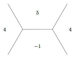
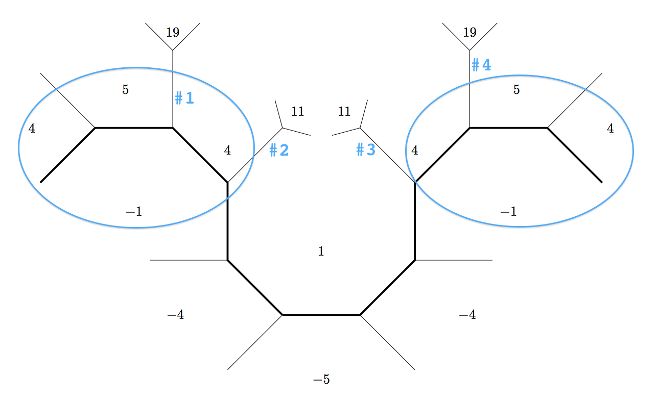
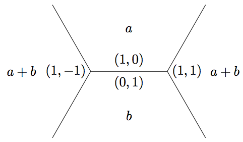
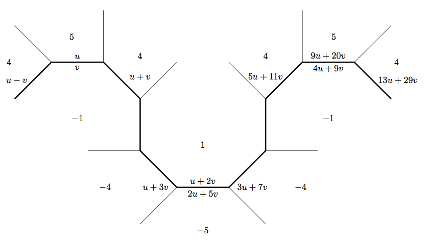
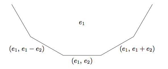
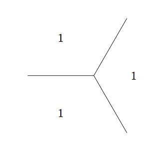
The base \((1, 0)\) and \((0, 1)\) take values \(a\) and \(b\) on the form in the Definition above and are part of a sequence with common difference \(h\). In fact, if we know the values \(a'\), \(b'\) and the difference \(h'\) at any base (edge in the topograph), the value \(a'b' - \left(\frac{1}{2}h'\right)^2\) is independent of the base and the direction (left or right) which determines the sign of \(h'\) and hence equal to the discriminant. To see this, first note the sign of \(h'\) is immaterial since it is squared. Also, consider the two other bases (edges) in the superbase. As in the proof of the climbing lemma, one base takes values \(a' = a\) and \(b' = a + b + h\) with common difference \(h' = 2a + h\) which gives
\begin{align*}
a'b' - \left(\frac{1}{2}h'\right)^2 &= a(a + b + h) - \frac{1}{4}\left(2a + h\right)^2 \\
&= a^2 + a b + a h - \left(a^2 + a h + \frac{1}{4} h^2\right) \\
&= ab - \left(\frac{1}{2}h\right)^2.
\end{align*}
Similarly the other base in the given superbase gives
\begin{align*}
a'b' - \left(\frac{1}{2}h'\right)^2 &= (a + b + h)b - \frac{1}{4}\left(2b + h\right)^2 \\
&= b^2 + a b + b h - \left(b^2 + b h + \frac{1}{4} h^2\right) \\
&= ab - \left(\frac{1}{2}h\right)^2.
\end{align*}
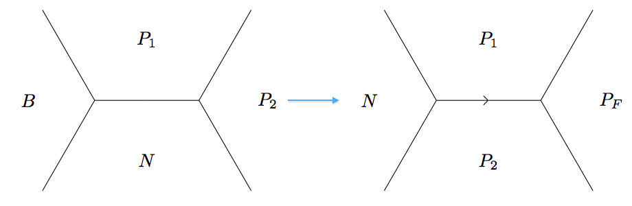
Having showed that there are no cycles when starting from a given superbase, our work in understanding the topograph is not complete. We haven't actually showed that we can get from one superbase to any other superbases within the topograph. To show this, we'll use the discriminant and the following.

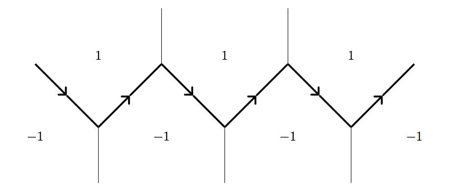
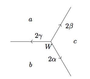
Definition: A superbase \(W\) is called a well if all the edges at \(W\) point away from \(W\).
\(\Box\)

Notice a well is dependent on the values, hence depends on the form \(f\). In a positive--valued topograph, we may find a well by traveling along the topograph in the opposite direction of the edges. Eventually, we must encounter a superbase where all arrows point out (as above), leaving us nowhere to travel and thus becoming our well. This is because, assuming the topograph is positive--valued, we can only decrease in value for so long (eventually the values must approach the minimum).

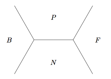
Lemma: (The Well Lemma) For a positive--valued form \(f\) and a well (with respect to \(f\)) \(W\), the three values \(f\) takes on the faces in \(W\) are the smallest values that \(f\) takes on the topograph.

Proof: Using the labels from the well in the definition above, the Arithmetic Progression Rule for our differences gives
\[2\alpha = b + c - a, \quad 2\beta = c + a - b, \quad 2\gamma = a + b - c\]
and solving,
\[a = \beta + \gamma, \quad b = \alpha + \gamma, \quad c = \beta + \alpha.\]
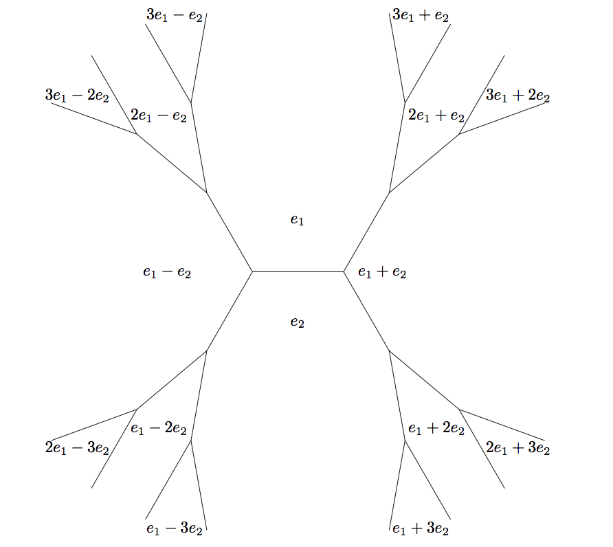
Let the superbase \(W = \left\{e_1, e_2, e_3\right\}\). Since \(W\) is a superbase, we may write any vector as
\[v = m_1 e_1 + m_2 e_2 + m_3 e_3\]
for \(m_1\), \(m_2\), \(m_3 \in \mathbf{Z}\). Also due to the fact that \(W\) is a superbase, \(e_1 + e_2 + e_3 = (0, 0)\) and so we may also write
\[v = (m_1 - k) e_1 + (m_2 - k) e_2 + (m_3 - k) e_3\]
for \(k \in \mathbf{Z}\). From this it is clear only the differences of the \(m_i\) matter. With this as our inspiration we write
\[f(v) = \alpha(m_2 - m_3)^2 + \beta(m_1 - m_3)^2 + \gamma(m_1 - m_2)^2,\]
a formula discovered by Selling.

To verify this, notice both sides of the equation are quadratic forms in \(v\) and
\begin{align*}
f(e_1) = a &= \beta + \gamma = \alpha \cdot 0^2 + \beta \cdot 1^2 + \gamma \cdot 1^2 \\
f(e_2) = b &= \alpha + \gamma = \alpha \cdot 1^2 + \beta \cdot 0^2 + \gamma \cdot (-1)^2 \\
f(e_3) = c &= \beta + \alpha = \alpha \cdot (-1)^2 + \beta \cdot (-1)^2 + \gamma \cdot 0^2.
\end{align*}
hence they must be equal since both sides are quadratics that agree on more than two points.

If two of the \(m_i\) are equal, then \(v\) must be an integral multiple of the third vector, hence the value \(f(v)\) will be at least as large as the value of \(f\) on the third vector. If not, all the differences must be non--zero (hence greater than or equal to \(1\) in absolute value, since integers), thus
\[f(v) \geq \alpha \cdot 1^2 + \beta \cdot 1^2 + \gamma \cdot 1^2\]
which is greater than or equal to each of \(a = \beta + \gamma\), \(b = \alpha + \gamma\), and \(c = \beta + \alpha\) since all of \(\alpha\), \(\beta\), and \(\gamma\) are non--negative. \(\Box\)

Corollary: The topograph is connected; one may travel along the topograph from any given superbase to any other.

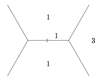
Proof: Using the same quadratic form \(f\) as we did to show the topograph had no cycles, we can show it is connected. Any arbitrary superbase is on the topograph, hence must be in some connected component of the topograph, but there may be more than one component. Since \(f\) is positive--valued, we must have some well in this component. But, by the above, the values at a well must be the absolute lowest values \(f\) takes on the topograph. This implies the well must take the values \(1\), \(1\), \(1\) and shows all superbases must be in the same component. \(\Box\)

From this point, we will concentrate on a special type of form relevant to our discussion. For a form \(f\) which takes both positive and negative values, but never \(0\), the topograph has a special path that separates the which separates the faces where takes a positive value and those where \(f\) takes a negative value.

Claim: If a form \(f\) takes both positive and negative values, but not zero, then there is a unique path of connected edges separating the positive and negative values. What's more, the values that occur on this river do so periodically.

Proof: Since the topograph is connected, there must be some edge where positive and negative values meet. As we proceed along adjacent edges, we can choose to follow a path of edges which will separate positive and negative (each subsequent value must be positive or negative, allowing us to "turn" left or right).
On first sight, there is no reason that this path should be unique. However, with the climbing lemma in mind, starting on the positive side of the path and moving away from the negative values, we must have only positive values. Using the logic of the climbing lemma instead with negative values, we similarly see that starting on the negative side and more away from the positive values will yield all negative numbers below the path. Hence nowhere above the path can positive and negative values meet and similarly below. Thus the path must be unique.

To show this path is periodic, we must utilize the discriminant. For each edge along the path, we have some positive value \(a\) and a negative \(b\) (by definition of the path) and the common difference \(h\). Thus the determinant \(D\) must be negative since the product \(ab\) is, hence
\[\left|D\right| = \left|ab\right| + \left(\frac{1}{2}h\right)^2.\]
Thus, both \(\left(\frac{1}{2}h\right)^2\) and \(\left|ab\right|\) are bounded by \(\left|D\right|\). So \(a\), \(b\) and \(h\) are bounded (by \(\left|D\right|\). Thus we have finitely many possible triples \((a, b, h)\), hence some value must be repeated in the path. This forces the path to be periodic since the triple starting from one triple \((a, b, h)\) determines next triple along the path and hence the entire path.

This path is so crucial that we give it it's own name.

Definition: If a form \(f\) takes both positive and negative values, but not zero, we call the path separating the positive and negative values the river. \(\Box\)

Thanks for reading, I'll make use of all this in a few days!

UpdateThis material is intentionally aimed at an intermediate (think college freshman/high school senior) audience. One can go deeper with it, and I'd love to get more technical off the post.

UpdateAll images were created with the tikz LaTeX library and can be compiled with native LaTeX if pgf is installed.

Conway's Topograph Part 2

This is the second (continued from Part 1) in a series of three blog posts. In the following we'll investigate a few properties of an object called Conway’s topograph. John Conway conjured up a way to understand a binary quadratic form – a very important algebraic object – in a geometric context. This is by no means original work, just my interpretation of some key points from his The Sensual (Quadratic) Form that I'll need for some other posts.


In the following, as mentioned in Part 1, "when referring to a base/superbase, we are referring to the lax equivalent of these notions."

To begin to form the topograph, note each superbase \(\left\{e_1, e_2, e_3\right\}\) contains only three bases
\[\left\{e_1, e_2\right\}, \left\{e_2, e_3\right\}, \left\{e_3, e_1\right\}\]
as subsets. Going the other direction, a base \(\left\{e_1, e_2\right\}\) can only possibly be contained as a subset of two superbases:
\[\langle e_1, e_2, (e_1 + e_2)\rangle, \langle e_1, e_2, (e_1 - e_2)\rangle.\]
With these two facts in hand, we can begin to form the geometric structure of the topograph. The interactions between bases and superbases (as well as the individual vectors themselves) give us the form. In the graph, we join each superbase (\(\bigcirc\)) to the three bases (\(\square\)) in it.
Each edge connecting two superbases (\(\bigcirc\)) represents a base and we mark each of these edges with a (\(\square\)) in the middle. Since each base can only be in two superbases, we have well--defined endpoints for each base (edge). Similarly, since each superbase contains three bases as subsets, each superbase (endpoint) has three bases (edges) coming out of it.
As we traverse each edge (base) surrounding a given vector (\(e_1\) above), we move from superbase (vertex) to superbase (vertex), and form a face. Starting from a base \(e_1, e_2\), traveling along each of the new faces encountered we begin to form the full (labeled) topograph below:
Notice the values of \(f\) on the combinations of \(e_1\) and \(e_2\) is immaterial to the above discussion, hence the shape of the topograph doesn't depend on \(f\).

If we know the values of \(f\) at some superbase, it is actually possibly to find the values of \(f\) at vectors (faces) we encounter on the topograph without actually knowing \(f\).

Claim: For vectors \(v_1, v_2\),
\[f(v_1 + v_2) + f(v_1 - v_2) = 2\left(f(v_1) + f(v_2)\right)\]
Proof: Exercise. (If you really can't get it, let me know in the comments.) \(\Box\)

This implies that if
\[a = f(v_1), \quad b = f(v_2), \quad c = f(v_1 + v_2), \quad d = f(v_1 - v_2)\]
then \(d\), \(a + b\), \(c\) form an arithmetic progression with common difference \(h\). This so--called Arithmetic Progression Rule allows us to mark each edge with a direction based on the value of \(h\). Hence if \(d < a + b < c\), we have \(h > 0\) and the following directed edge:
Obviously starting from a base \(e_1, e_2\), one wonders if it is possible to move to any pair \((x, y)\) with \(x\) and \(y\) coprime along the topograph. It turns out that we can; the topograph forms a structure called a tree, and all nodes are connected.

Lemma: (Climbing Lemma) Given a superbase \(Q\) with the surrounding faces taking values \(a\), \(b\), and \(c\) as below, if the \(a\), \(b\) and the common difference \(h\) are all positive, then \(c\) is positive and the other two edges at \(Q\) point away from \(Q\).
Proof: First \(c\) is positive because \(h = c - (a + b)\), hence \(c = a + b + h > 0\). The two other edges at \(Q\) have common differences \((a + c) - b\) and \((b + c) - a\). Since \(c = a + b + h\) is greater than both \(a\) and \(b\), these differences are positive. \(\Box\)

Notice also that this establishes two new triples \((a, a + b + h, 2 a + h)\) and \((b, a + b + h, 2 b + h)\) that continue to point away from each successive superbase and hence climb the topograph. We can use this lemma (along with a specific form) to show that there are no cycles in the topograph, i.e. the topograph doesn't loop back on itself.

Consider the form which takes the following values at a given superbase:
Due to the symmetry, we may consider traveling along an edge in any direction from this superbase identically. Picking an arbitrary direction, we reach the following superbase:
Since the values must increase indefinitely as laid out by the climbing lemma, the form can't loop back on itself; if it were to, it would need to loop back to a smaller value. Since this holds in all directions from the original well, there are no cycles.

Follow along to Part 3.

Update: This material is intentionally aimed at an intermediate (think college freshman/high school senior) audience. One can go deeper with it, and I'd love to get more technical off the post.

Update: All images were created with the tikz LaTeX library and can be compiled with native LaTeX if pgf is installed.

Conway's Topograph Part 1

This is the first in a series of three blog posts. In the following we'll investigate a few properties of an object called Conway’s topograph. John Conway conjured up a way to understand a binary quadratic form – a very important algebraic object – in a geometric context. This is by no means original work, just my interpretation of some key points from his The Sensual (Quadratic) Form that I'll need for some other posts.


Definition: A binary quadratic form \(f\) is an equation of the form:
\[f(x, y) = A x^2 + H x y + B y^2.\]
That is, a function of two variables which is homogeneous of degree two. The coefficients \(A\), \(H\), and \(B\) and variables \(x\) and \(y\) are often real numbers, rational numbers or integers. \(\Box\)

When we require the coefficients \(A\), \(H\), and \(B\) as well as the variables \(x, y\) to be integers, we get an integer--valued form. In his Disquisitiones Arithmeticae, Gauss asked (and largely answered) the fundamental question: what integer values can each form take? For example, you may have seen the form
\[f(x, y) = x^2 + y^2,\]
where it was determined that the only primes (Gaussian primes) occuring were \(2\) and those odd primes congruent to 1 modulo 4.

As each form \(f\) is homogenous degree two, \(f(\lambda x, \lambda y) = \lambda^2 f(x, y)\). As a result, if we can understand the values of \(f\) for pairs \((x, y)\) which don't share any factors, we can understand the entire set of values that \(f\) takes. Also, letting \(\lambda = -1\), there is no change in the value of \(f\) since \(\lambda^2 = 1\), hence it suffices to think of \(v = (x, y)\) as \(\pm v\), i.e. \(\left\{(x, y), (-x, -y)\right\}\).

For integers \(x\) and \(y\), any point \((x, y)\) can be expressed as an integral linear combination of the vectors \(e_1 = (1, 0)\) and \(e_2 = (0, 1)\). So if we like, we can express all relevant inputs for \(f\) in terms of two vectors. However, instead considering \(e_2 = (1, 1)\), we have
\[(x - y) \cdot e_1 + y \cdot e_2 = (x, y)\]
and realize a different pair \(e_1, e_2\) which again yield all possible integer valued vectors as integral linear combinations.

Definition: A strict base is an ordered pair \((e_1, e_2)\) whose integral linear combinations are exactly all vectors with integer coordinates. A lax base is a set \(\left\{\pm e_1, \pm e_2\right\}\) obtained from a strict base. \(\Box\)

Definition: A strict superbase is an ordered triple \((e_1, e_2, e_3)\), for which \(e_1 + e_2 + e_3 = (0, 0)\) and \((e_1, e_2)\) is a strict base (i.e., with strict vectors), and a lax superbase is a set \(\langle\pm e_1, \pm e_2, \pm e_3\rangle\) where \((e_1, e_2, e_3)\) is a strict superbase. \(\Box\)

For our (and Conway's) purposes, it is useful to consider the lax notions and leave the strict notions as an afterthought since a binary quadratic form is unchanged given a sign change. From here forward, for a vector \(v\), we use the notation \(v\) interchangeably with \(\pm v\) and when referring to a base/superbase, we are referring to the lax equivalent of these notions.

Follow along to Part 2.

Update: This material is intentionally aimed at an intermediate (think college freshman/high school senior) audience. One can go deeper with it, and I'd love to get more technical off the post.

Wednesday, August 17, 2011

The Lesson V8 Can Teach Python and Other Dynamic Languages

Being unable to completely give up math for computers, I am naturally drawn to Project Euler and as a result solved a ridiculous number of the problems posted there while learning Python. A few months ago (March 13), after reading Secrets of a Javascript Ninja, I decided to begin converting my solutions to Javascript. A month and a half later I came back to it, and then finally two months after that, I began to take it seriously.

After making this decision, I noticed the prime Sieve of Eratosthenes was mighty fast when I ran it in Chrome, maybe even faster than my beloved Python. I tabled the thought for a little, but never really forgot it. So a few weeks ago (early August 2011), I finally got a working install of node running on my machine and was able to make more of this thought. (I say finally installed because on two previous tries I gave up because of conflicts with my version of gcc, coupled with the fact that I had no good reason to use node.)

When I originally did the conversion, I had skipped problem 8, because my implementation required pulling in the problem data as text from a file. While hanging out with Boris and Eric from on the Chrome Developer Relations team, I decided to give it another go on node (xhr requests not allowed) and found it to be quite simple with readFileSync in the node native fs module. After witnessing this, over this weekend, I decided to harness the power of V8 -- the Javascript engine that powers Chrome and node -- and run all my scripts locally with node. So over a two day period, I hack-hack-hacked my way into converting the Python solutions for problems 11 through 50 (the remaining unconverted) into their Javascript equivalents, while also converting a good portion of my hefty functions module.

Once this was done, I had also found I could replace most of the nice parts about Python with my own equivalent. For example, I was able to replace functionality I needed from the Python set datatype with
function uniq(arr) {
  var result = {};
  for (var i = 0, val; val = arr[i]; i++) {
    result[val] = true;
  }

  return Object.keys(result);
};
and I was able to replace the (amazingly) useful Python handling of long integers with a non-native node package called bigint that uses libgmp among other usings. Of course, for Python's secret sauce -- the list comprehension -- I was able to substitute enough filter, reduce and map statements to almost make it seem like I had never left Pythonland. After doing all this, I also ended up writing my own operator.js to replace the wonderful Python native module operator, and my own timer.js to stand in for the Python native module time.

Finally, I had working code and could do a side by side comparison of V8 and the Python interpreter. Update: I added a column for PyPy, a just in time implementation of Python. Here is what I found (averaging the runtime over 10 separate calls to each function, the results are):

ProblemAnswerPythonJavascriptRatio (PY/JS)PyPy
1*2331681804ms1215ms1.48385ms
2*4613732247ms102ms2.4285ms
3*68574725ms1508ms3.13582ms
49066098708ms149ms58.44282ms
5*232792560136ms186ms0.73114ms
6*2516415010ms4ms2.506ms
7104743656ms12ms54.6711ms
8*4082418045ms5014ms3.607042ms
931875000610ms3ms203.338ms
101429138289226628ms167ms39.69116ms
117060067449ms2ms24.5011ms
12765765005127ms203ms25.26100ms
13*55373762301795ms10710ms0.171423ms
148377995572ms1712ms3.25362ms
15*13784652882054ms18ms3.0055ms
16*13661844ms265ms6.96462ms
172112487ms4ms21.757ms
18*10742291ms1790ms1.281090ms
19*1712254ms336ms6.71342ms
20*6481061ms9154ms0.12374ms
213162618910ms1038ms18.22728ms
22871198282188ms7ms26.868ms
23417987183318ms1120ms74.391295ms
24*2783915460206ms210ms0.98139ms
2547825865ms35ms167.57232ms
2698328ms18ms1.564ms
27-59231645738ms22536ms28.6528288ms
28*6691710018509ms1037ms8.21981ms
299183184ms96ms1.9220ms
3044383952167ms1037ms50.31877ms
31736829606ms257ms37.38154ms
3245228206888ms12096ms17.104266ms
33100300ms6ms50.0015ms
34407307462ms2447ms3.05247ms
35558617ms848ms10.16242ms
36872187189788ms2183ms86.943532ms
377483172389022ms71845ms33.2561551ms
38932718654506ms10ms50.6012ms
39840178ms6ms29.6712ms
40*210326ms202ms1.61119ms
4176524132627ms133ms19.7565ms
4216265ms7ms9.298ms
431669533489038ms2ms19.002ms
445482660384013ms27744ms13.846621ms
45*153377680517ms4ms4.258ms
4657772864ms202ms14.1865ms
47134043400967ms12838ms31.234425ms
48911084670046ms16ms2.886ms
49296962999629115ms8ms14.3813ms
509976513277ms80ms40.9651ms
*These were very quick to run, so the runtimes are the time taken to run 10000 times.

As you'll notice, standard Python gets its butt kicked. I was kind of saddened by this, but in the end, just giddy that our web is faster because of it (90% of my life is digital) and also that we can do scripting faster on the server side (attribute to Boris Smus) because of the node project (thanks Ryan Dahl).

Standard Python is actually slower in 46 of the 50 problems. In 28 of the 46 node is faster by a factor of 10 or greater, in 9 of those 28 by a factor of 50 or greater and in 2 of the 9 by a factor of 100 or greater! The only 4 in which Python was faster were from the n = 10000 sample. In fact, I was able to pinpoint exactly why:
  • #5 - My own Javascript implementation of gcd is slower than the native (from fractions import gcd) Python library (resulting in a difference of 50 ms over 10000 iterations)
  • #13 - The node package bigint is slower than the Python native long int (Javascript is slower by a factor of 6)
  • #20 - The node package bigint is slower than the Python native long int (Javascript is slower by a factor of 8.5)
  • #24 - Having to perform two slices is slower in Javascript than in Python and there is no good way to just remove one element (resulting in a difference of 4 ms over 10000 iterations; a little bit about that here)
So what, you ask, is that lesson I speak of? Well, Javascript didn't used to be this fast. How did it get that way? The brilliant and inspired people behind V8 rethought the Javascript compile steps and after much work, we now have code that is closer to the metal (attribute to: Eric Bidelman, i.e. closer to machine code) than we had ever had before. The use of just-in-time compilation and other incredible techniques has taken a formerly slow and clunky language (Javascript) which was used well beyond its original intended scope, and turned it into a damn fast dynamic language. Hopefully, this movement will make its way to Python and other dynamic languages and we can all have our code end up this close to the metal.

Update: In response to the comments, I ran the same code on the same machine, but with PyPy in place of Python. This is the direction I hope standard Python goes in and commend the guys pumping out faster and faster just in time implementations over at PyPy. I went through and counted 20 node wins, 29 PyPy wins and 1 tie. (I reserve the right to update the post with more detailed metrics.) While I do commend them, the results don't really belong in this post because PyPy is still an offshoot. (However, as I understand, they both have ties to C, as PyPy uses GCC to compile to bytecode and V8 is written in C++. Feel free to supplement my knowledge in the comments.)

Update: All benchmarking was run on my Mac Pro Desktop with a 3.2 GHz Quad-Core Intel Xeon processor and 4 cores for a total of 12 GB 1066 MHz DDR3 memory. I used Python version 2.6.1, node version 0.4.9, and PyPy version 1.5 (running on top of Python 2.7.1 with GCC 4.0.1).